Global Fishing Watch is committed to increasing the transparency of the world’s fisheries. Open science is a key component of this message and we strive to make as much data and code publicly available as possible. In addition to our map, data are available in several formats, including as downloadable files, BigQuery tables, and Google Earth Engine image collections. We recognize, however, that working with these data formats can be tricky and requires some knowledge of programming. In this post, we provide example code for working with the public Global Fishing Watch data in Google Earth Engine.
Google Earth Engine
Google Earth Engine (GEE) is a planetary-scale platform for Earth science data & analysis. GEE combines a multi-petabyte catalog of satellite imagery and geospatial datasets with planetary-scale analysis capabilities and makes it available for scientists, researchers, and developers to detect changes, map trends, and quantify differences on the Earth’s surface. The primary way to interact with the GEE platform is via the Code Editor, a web-based IDE for writing and running scripts. Client libraries also provide Python and JavaScript wrappers around the web API.
In the following examples, we’ll demonstrate how to use GEE to load, filter, summarize, and export our public fishing effort dataset. The examples are done in JavaScript using the Code Editor and the complete script for this tutorial is available here.
Examples
Global Fishing Watch data are hosted on GEE as two separate ImageCollections, one for vessel hours and one for fishing hours. The fishing hours collection contains daily rasters of fishing effort measured in hours of inferred fishing activity per square kilometer and can be imported using the asset ID “GFW/GFF/V1/fishing_hours”. You can also browse GEE’s extensive data catalog and import layers directly into your scripts by using the “Search places and datasets…” search bar at the top of the page.
// Import GFW data
var gfw = ee.ImageCollection('GFW/GFF/V1/fishing_hours');
Each image in the collection contains the effort for a given flag state and day, with one band for the fishing activity of each of the following gear types:
Bands:
0: drifting_longlines
1: fixed_gear
2: other_fishing
3: purse_seines
4: squid_jigger
5: trawlers
Example 1: Total fishing effort over date range
For our first example, we’ll create a map of total global fishing effort in 2016. Each image in the collection has a country property in its metadata containing the ISO3 country code for the flag state represented in the image. The .filterMetadata()function allows us to filter the collection by the country property and explore specific countries of interest. To examine total global fishing effort, we can use the "WLD" code. We’ll also use .filterDate() to extract only effort data for 2016. Note that the second date is exclusive, meaning if we used 2016-12-31 we would accidentally omit it from our analysis.
// Filter by "WLD" to get all global fishing effort rasters in 2016
var effort_all = gfw
  .filterMetadata('country', 'equals', 'WLD')
  .filterDate('2016-01-01','2017-01-01');
Next, we use .sum() to flatten the collection to a single image where each pixel is the sum of all corresponding pixels in the collection. This aggregation is applied to each band (gear type) individually.
// Aggregate 2016 collection to single image of global fishing effort
var effort_2016 = effort_all.sum();
We now have a multi-band image where each band contains the total global fishing effort for that gear type. We can isolate global effort for each gear type, like trawlers, by selecting the desired image band.
// Select band of global trawling effort
var all_trawling_2016 = effort_2016.select('trawlers');
Finally, to look at total fishing effort across all gear types, we use .reduce(ee.Reducer.sum()) to aggregate the gear types into a single band. We’ll also mask any pixels without fishing hours.
// Sum bands to get total effort across gear types
var effort_all_2016 = effort_2016.reduce(ee.Reducer.sum());

// Mask out pixels with no effort
effort_all_2016 = effort_all_2016.mask(effort_all_2016.gt(0));
We can now add this layer to our map in GEE, specifying a custom color ramp.
// Add the total fishing effort layer
Map.addLayer(effort_all_2016,{palette: ['0C276C', '3B9088', 'EEFF00', 'ffffff']});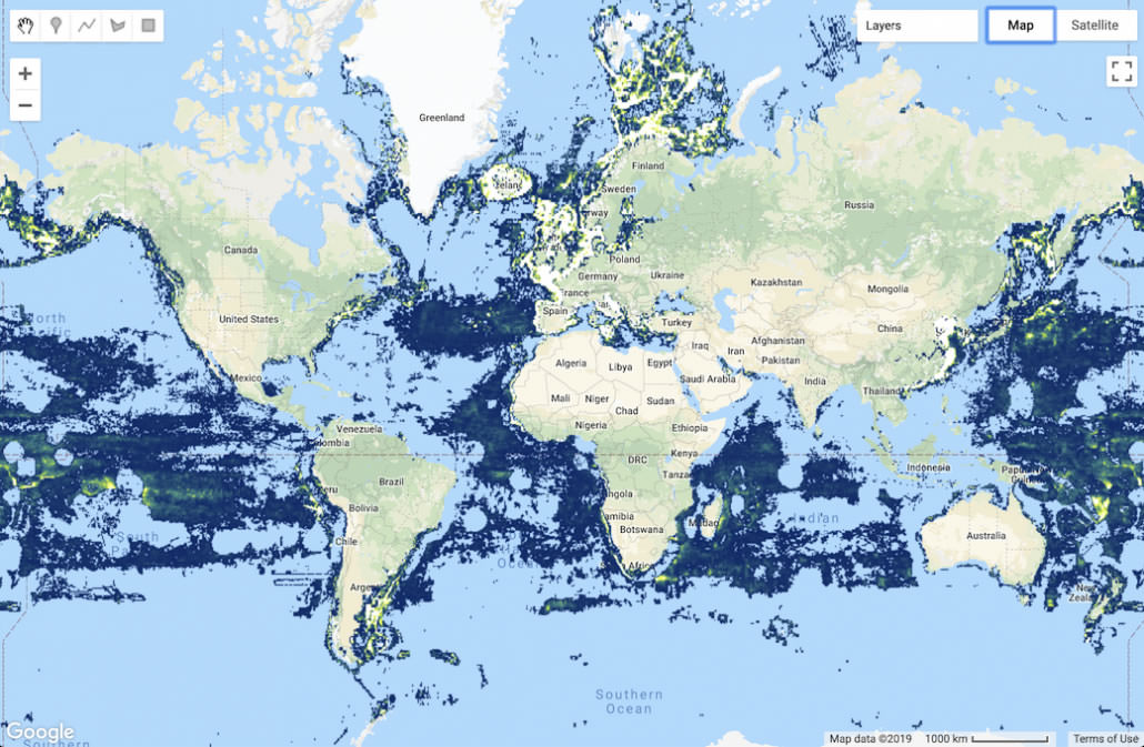
Figure 1: Global fishing effort (hours per square kilometer) in 2016
Example 2: Fishing effort by flag state
Exploring fishing effort for a specific flag state can be done in much the same way as Example 1. However, this time we’ll define a function that we can use to aggregate data for a given flag state and date range.
// Define a function to filter/aggregate for a specific flag state and date range
var flag_totals = function(flag, start_date, end_date) {
  var effort_flag = gfw
  .filterMetadata('country', 'equals', flag)
  .filterDate(start_date, end_date)
  .sum();
  return ee.Image(effort_flag);
};
We can now run our function to extract the fishing effort for any flag state over any time range. For example, to get China’s fishing effort in 2016 we do the following:
// Apply function to China
var china = flag_totals('CHN','2016-01-01','2017-01-01');

// Calculate total effort across gear types
var china_all = china.reduce(ee.Reducer.sum());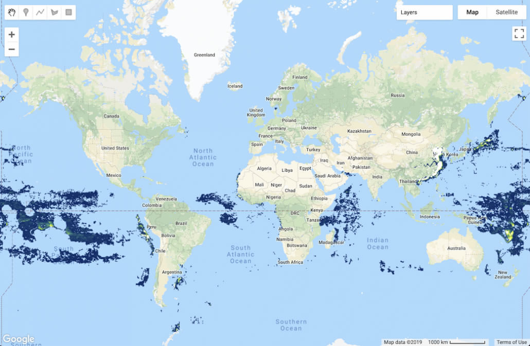
Figure 2: Fishing effort (hours per square kilometer) by Chinese-flagged vessels in 2016
As in Example 1, we can also use .select() to pull out China’s fishing effort for individual gear types, in this case drifting longlines.
// Isolate drifting longline effort

china_drift_lines = china.select('drifting_longlines');
Example 3: Fishing effort in a region
It is often desirable to examine fishing effort within a specific area of the ocean (e.g. exclusive economic zone, marine protected area). To demonstrate this in GEE, let’s import the World Database on Protected Areas (which you can find using the Code Editor search bar) as a FeatureCollection of polygons and select all protected areas located 100% in the ocean.
// Import the WDPA FeatureCollection and select marine protected areas
var wdpa = ee.FeatureCollection('WCMC/WDPA/current/polygons');
var mpas = wdpa.filterMetadata('MARINE', 'equals', '2');
Next, we can clip our image of 2016 global fishing effort to the bounds of all polygons in the mpas collection.
// Clip our total effort layer to the bounds of the MPA collection
var mpa_effort_2016 = effort_all_2016.clipToCollection(mpas);
We don’t need to mask pixels without fishing hours in our MPA layer before plotting because the effort_all_2016 layer is already masked.
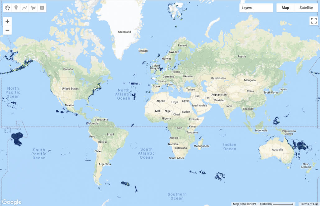
Figure 3: Fishing effort (hours per square kilometer) within marine protected areas in 2016.
We can see that fishing occurred within the boundaries of MPAs all around the world. It is important to note that although some illegal fishing is likely captured in this image, many MPAs allow fishing in some capacity or within certain areas.
Additionally, we could explore fishing in a single MPA by further filtering the mpas collection and clipping the image to the polygon.
// Extract the PIPA polygon from the MPA collection and use it to clip our total effort layer
var pipa = wdpa.filterMetadata('WDPAID', 'equals', 220201);
var pipa_effort_2016 = effort_all_2016.clip(pipa.geometry());
If you would like to work with your own vector data, such as a shapefile outlining your study area, you can import table data to a GEE asset and load it as a FeatureCollection.
Example 4: Exporting images to Google Drive
GEE is a powerful tool for analyzing the full catalog of our public fishing effort data. However, you may often wish to export your results in order to work with them in another program, such as R or QGIS. Fortunately, GEE provides several ways to export your work, including directly to Google Drive.
By default, GEE will export only the portion of the image that is visible in the map viewer. To avoid this, we must specify a specific geometry, such as the pipa polygon from above (using pipa.geometry()). In this case, we’re interested in a global map so we’ll create a rectangle that covers the entire world (Note: we use 179.999 otherwise Earth Engine only exports a small sliver).
// Define a geometry to use as the region of interest for export
var bounds = ee.Geometry.Rectangle([-179.999, -90, 180, 90], 'EPSG:4326', false)
Finally, we export the image to Google Drive, specifying the region to export using bounds and the scale (in meters) of the output image’s cells. In this case we use 1000, which is the default output scale and the same as the native resolution of the data.
Export.image.toDrive({
  image: effort_2016, // image to export
  description: 'global_effort_2016', // name of export job
  scale: 1000, // scale (meters) of the output
  region: bounds, // region to export
  maxPixels: 1e13 // maximum number of pixels to allow in export.
});
After running your script to export an image, it is necessary to navigate to the Tasks tab on the right side of the Code Editor and press the “Run” button next to the name of your export job (the description field of the export command). Once complete, the exported GeoTIFF will be in your “My Drive” folder on Google Drive. If the output image is large, the image is split into tiles. The filename of each tile will be in the form baseFilename-yMin-xMin where xMin and yMin are the coordinates of each tile within the overall bounding box of the exported image.
Conclusion
Google Earth Engine is a great tool for analyzing our public data. It provides a powerful platform to work with the large amounts of public data we make available, as well as an extensive catalogue of other environmental and remote sensing datasets to use in your analyses. While there can be a a fairly steep learning curve for GEE, we hope that this tutorial will help you get started.
Additional resources
- GEE Developers Google Group – The primary forum for asking and answering technical questions related to GEE. The group is very active and you can often find an answer to your question by searching previous questions.
- GEE API Documentation – Official GEE documentation, including how-to guides, technical reference, and tutorials.