Introduction
Global Fishing Watch is committed to increasing the transparency of the world’s fisheries. Open science is a key component of this message and Global Fishing Watch strives to make as much data and code publicly available as possible. In addition to our map, these data are a way to provide users with a fine scale picture of global fishing effort that they can use for research and policy making. However, we recognize that working with these data formats can be tricky for some users, as a degree of programming knowledge is required. In this post, we provide example R code for working with our downloadable public data, which is available for anyone to download by registering on the Datasets and Code page of our website.
R
R is a scientific programming language and a popular tool among our users for processing and visualizing Global Fishing Watch data. The following code snippets provide examples for working with our downloadable fishing effort data in R in order to calculate, plot, and export various maps of fishing effort.
We will use several R packages to work with the data. The tidyverse package contains several helpful packages for data manipulation (dplyr, tidyr, readr) and plotting (ggplot2). The furrr package is useful for running operations in parallel, lubridate is great for working with dates, and the sf and raster packages are designed for working with vector and raster data, respectively, in R. There are also a few additional mapping packages that are helpful for plotting. If you do not already have these packages installed you can do so with the install.packages() function.
# Load packages
library(tidyverse) # for general data wrangling and plotting
library(furrr) # for parallel operations on lists
library(lubridate) # for working with dates
library(sf) # for vector data
library(raster) # for working with rasters
library(maps) # additional helpful mapping packages
library(maptools)
library(rgeos)
Downloadable data
Daily fishing effort data are available for download in the following two formats:
- Daily Fishing Effort and Vessel Presence at 100th Degree Resolution by Flag State and GearType, 2012-2016
- Daily Fishing Effort and at 10th Degree Resolution by MMSI, 2012-2016
Upon downloading each dataset, users will receive a .zip file containing a folder named fishing_effort (or fishing_effort_byvessel) that itself contains the data readme.txt file and the daily_csvs folder. The daily csvs are named according to the YYYY-MM-DD.csv format. The files generally increase in size over time due to the higher number of satellites receiving AIS data. Since we will be using both datasets, let’s rename the fishing_effort folder to fishing_effort_byflag and then store both the fishing_effort_byflag and fishing_effort_byvessel folders within a directory called fishing_effort.
Data containing details on the fishing vessels included in the fishing effort datasets are also available. These data can be used in conjunction with the “Daily Fishing Effort and at 10th Degree Resolution by MMSI” data to explore vessel and fleet characteristics and provide details (gear type, flag state, etc.) for the MMSI being analyzed.
Shapefiles
Shapefiles of land and Exclusive Economic Zone (EEZ) boundaries are useful for providing context to maps of fishing effort. For this analysis, we’ll use a land shapefile from the maps R package and an EEZ shapefile from MarineRegions.org. We’ll also load/convert both of these shapefiles to sf objects. The sf R package is a great package for working with vector data stored in dataframes, providing numerous functions for performing spatial operations.
# World polygons from the maps package
world_shp <- sf::st_as_sf(maps::map("world", plot = FALSE, fill = TRUE))

# Load EEZ polygons
eezs <- read_sf('~/data/shapefiles/World_EEZ_v10_20180221/', layer = 'eez_v10') %>%
  filter(Pol_type == '200NM') # select the 200 nautical mile polygon layer
Daily Fishing Effort and Vessel Presence at 100th Degree Resolution by Flag State and GearType, 2012-2016
Let’s start by exploring our daily fishing effort and vessel presence dataset, which provides a very fine-scale view of global fishing behavior. We’ll load a single year of data (2016) and produce various summaries and maps of fishing effort.
Importing data
To get started, we first tell R where the fishing_effort folder containing the downloaded datasets is located. For this tutorial, we saved the fishing_effort folder within a data/gfw-public-data/ directory in our user folder. If you decide to save the fishing_effort folder in another location, simply change the location of data_dir in the code below.
We can then create a dataframe (or “tibble”) of dates and associated filenames.
# Specify location of data directory
data_dir <- '~/data/gfw-public-data/fishing_effort/'

# Create dataframe of filenames dates and filter to date range of interest
effort_files <- tibble(
  file = list.files(paste0(data_dir, 'fishing_effort_byflag'),
                    pattern = '.csv', recursive = T, full.names = T),
  date = ymd(str_extract(file,
                         pattern = '[[:digit:]]{4}-[[:digit:]]{2}-[[:digit:]]{2}')))
The full 2012-2016 dataset is nearly 20 Gb, so you’ll likely want to filter the files to the date range you’re interested in working with. In this case, we’ll examine all fishing effort in 2016.
# Generate a vector of dates of interest using ymd from lubridate
effort_dates <- seq(ymd('2016-01-01'), ymd('2016-12-31'), by='days')

# Filter to files within our date range of interest
effort_files <- filter(effort_files, date %in% effort_dates)
Next, after selecting all the 2016 files, we load the csv files of fishing effort and add variables for the year and month. We can use the future_map_dfr() function from the furrr package to read in the data from the csv files in parallel. This can take time and require a lot of memory depending on how many files you’re interested in working with. For reference, the 2016 data contains ~98 million rows and occupies over 7 Gb of memory.
# Read in data (uncomment to read in parallel)
plan(multiprocess) # Windows users should change this to plan(multisession)
effort_df <- furrr::future_map_dfr(effort_files$file, .f = read_csv)

# Add date information
effort_df <- effort_df %>%
  mutate(year  = year(date),
         month = month(date))
Adjusting data resolution
We now have a data frame (effort_df) containing all the fishing effort data for 2016 that we can summarize in various ways. The native data are at a resolution of 0.01 degrees. This resolution is great for fine scale analyses, however, we’re interested in making global maps and 0.01 degrees is a much finer resolution than necessary. So, before doing any summaries, let’s adjust the resolution of the data by calculating new values for lat_bin and lon_bin at our desired resolution of 0.25 degrees.
# Specify new (lower) resolution in degrees for aggregating data
res <- 0.25

# Transform data across all fleets and geartypes
effort_df <- effort_df %>%
  mutate(
    # convert from hundreths of a degree to degrees
    lat_bin = lat_bin / 100,
    lon_bin = lon_bin / 100,
    # calculate new lat lon bins with desired resolution
    lat_bin = floor(lat_bin/res) * res + 0.5 * res,
    lon_bin = floor(lon_bin/res) * res + 0.5 * res)
We can now aggregate the data to generate results gridded at 0.25 degrees instead of 0.01.
# Re-aggregate the data to 0.25 degrees
effort_df <- effort_df %>%
  group_by(date, year, month, lon_bin, lat_bin, flag, geartype) %>%
  summarize(vessel_hours = sum(vessel_hours, na.rm = T),
            fishing_hours = sum(fishing_hours, na.rm = T),
            mmsi_present  = sum(mmsi_present, na.rm = T))
Aggregating the data to the new resolution considerably reduced the size (~8.2 million rows) and memory usage (1.4 Gb) of effort_df and subsequent calculations will now run much faster.
We’re now ready to examine fishing effort patterns in various ways, which we can do by grouping the calculations by different combinations of variables.
Mapping fishing effort
Total global fishing effort in 2016
First, let’s calculate the total global fishing effort in 2016 across all flag states and gear types by grouping our calculations by lat_bin and lon_bin. We’ll exclude cells with fewer than 24 fishing hours and log transform the total fishing hours to better visualize the results.
# Aggregate data across all fleets and geartypes
effort_all <- effort_df %>%
  group_by(lon_bin,lat_bin) %>%
  summarize(fishing_hours = sum(fishing_hours, na.rm = T),
            log_fishing_hours = log10(sum(fishing_hours, na.rm = T))) %>%
  ungroup() %>%
  mutate(log_fishing_hours = ifelse(log_fishing_hours <= 1, 1, log_fishing_hours),
         log_fishing_hours = ifelse(log_fishing_hours >= 5, 5, log_fishing_hours)) %>%
  filter(fishing_hours >= 24)
The effort_all dataframe now contains a single value per grid cell representing the total fishing hours in that grid cell in 2016. We’re now ready to make a map of our data using the ggplot() function from the ggplot2 package. We use geom_sf() to add our land and EEZ layers and geom_raster() to add our gridded fishing effort layer.
# Linear green color palette function
effort_pal <- colorRampPalette(c('#0C276C', '#3B9088', '#EEFF00', '#ffffff'),
                               interpolate = 'linear')

# Map fishing effort
p1 <- effort_all %>%
  ggplot() +
  geom_sf(data = world_shp,
          fill = '#374a6d',
          color = '#0A1738',
          size = 0.1) +
  geom_sf(data = eezs,
          color = '#374a6d',
          alpha = 0.2,
          fill = NA,
          size = 0.1) +
  geom_raster(aes(x = lon_bin, y = lat_bin, fill = log_fishing_hours)) +
  scale_fill_gradientn(
        "Fishing Hours",
        na.value = NA,
        limits = c(1, 5),
        colours = effort_pal(5), # Linear Green
        labels = c("10", "100", "1,000", "10,000", "100,000+"),
        values = scales::rescale(c(0, 1))) +
  labs(fill  = 'Fishing hours (log scale)',
       title = 'Global fishing effort in 2016') +
  guides(fill = guide_colourbar(barwidth = 10)) +
  gfw_theme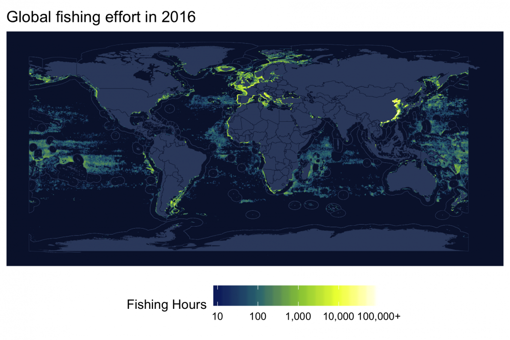
Fishing effort by gear type
Next, to examine fishing effort by gear type, we can simply summarize effort_all again, this time grouping by geartype in addition to lon_bin and lat_bin.
# Aggregate data by geartype across all fleets
effort_gear <- effort_df %>%
  group_by(lon_bin,lat_bin, geartype) %>%
  summarize(fishing_hours = sum(fishing_hours, na.rm = T),
            log_fishing_hours = log10(sum(fishing_hours, na.rm = T))) %>%
  ungroup() %>%
  mutate(log_fishing_hours = ifelse(log_fishing_hours <= 1, 1, log_fishing_hours),
         log_fishing_hours = ifelse(log_fishing_hours >= 5, 5, log_fishing_hours)) %>%
  filter(fishing_hours >= 24)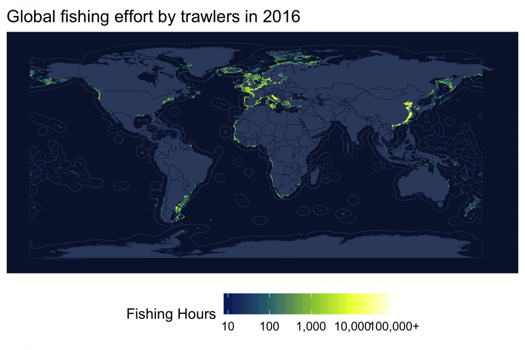
Fishing effort by flag state
Finally, we can examine the fishing effort of a specific flag state in the same manner. Let’s look at Chinese Taipei.
# Aggregate data by geartype across all fleets
effort_flag <- effort_df %>%
  filter(flag %in% c('TWN')) %>%
  group_by(lon_bin, lat_bin, flag) %>%
  summarize(fishing_hours = sum(fishing_hours, na.rm = T),
            log_fishing_hours = log10(sum(fishing_hours, na.rm = T))) %>%
  ungroup() %>%
  mutate(log_fishing_hours = ifelse(log_fishing_hours <= 1, 1, log_fishing_hours),
         log_fishing_hours = ifelse(log_fishing_hours >= 5, 5, log_fishing_hours)) %>%
  filter(fishing_hours >= 24)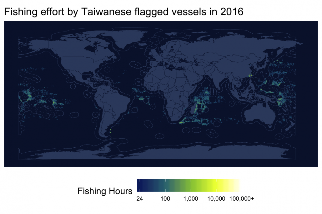
Fishing effort within a region
Often we are interested in examining fishing effort within a specific region, such as a marine protected area or a country’s EEZ. While our public data includes information on flag state, this is not the same as fishing location – vessels can fish outside the waters of their flag state. Thus, we need to use the spatial location of the effort, not the flag state. To accomplish this, we first need a polygon for the region of interest. In some cases, this polygon could be a simple bounding box.
For this example, we’ll examine fishing effort within the Peruvian EEZ in 2016. First, let’s extract Peru’s EEZ from our eezs object. We’ll also calculate a bounding box around Peru’s EEZ to constrain our maps.
# Select Peru EEZ
per <- eezs %>%
  filter(ISO_Ter1 == 'PER' & Pol_type == '200NM') %>%
  dplyr::select(ISO_Ter1, geometry)

# Get bounding box for Peru EEZ
per_bbox <- sf::st_bbox(per)
Next, we need to convert our effort_all dataframe to an sfobject, specifying which variables represent the coordinates, in order to perform spatial operations between our fishing effort data and our EEZ. Doing this requires defining a coordinate reference system (crs) for the data, and this crs must match the crs of the per polygon. In this case, both data are in decimal degrees using the WGS 1984 map datum and we can just set the crs of the effort data equal to the crs of the Peru shapefile.
# Convert effort data frame to sf object
effort_all_sf <- st_as_sf(effort_all,
                       coords = c("lon_bin", "lat_bin"),
                       crs = st_crs(per))
Next, we’ll use a spatial join between the effort_all_sf and per dataframes. The join adds the ISO_Ter1 variable to the effort_all_sf dataframe, allowing us to then filter the data to only include points within the Peruvian EEZ (ISO_Ter1 == 'PER'). Lastly, for plotting reasons, we remove the geometry column that was added when we converted the data to an sf object.
# Filter effort data to within the Peruvian EEZ
per_effort <- effort_all_sf %>%
  sf::st_join(per, join = st_intersects) %>% # use a spatial join
  filter(ISO_Ter1 == 'PER') %>% # filter only datapoints within Peruvian EEZ
  bind_cols(st_coordinates(.) %>% as.data.frame()) %>%
  rename(lat_bin = Y,
         lon_bin = X) %>%
  st_set_geometry(NULL)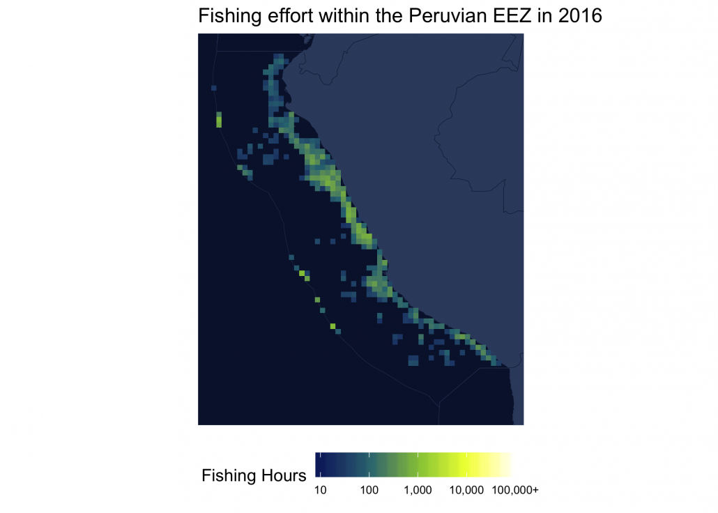
Daily Fishing Effort and at 10th Degree Resolution by MMSI, 2012-2016
So far, we’ve mapped fishing effort aggregated across many vessels for a given flag state or gear type. Let’s now use our Daily Fishing Effort at 10th Degree Resolution by MMSI, 2012-2016 data to map the fishing effort of specific vessels. In particular, let’s map the total 2016 fishing effort for the top three MMSI operating in the Peruvian EEZ.
To get started, we load and filter the data in the same fashion as before:
# Create dataframe of filenames dates and filter to date range of interest
mmsi_effort_files <- tibble(
  file = list.files(paste0(data_dir, 'fishing_effort_byvessel'),
                    pattern = '.csv, recursive = T, full.names = T),
  date = ymd(str_extract(file,
                         pattern = '[[:digit:]]{4}-[[:digit:]]{2}-[[:digit:]]{2}'))) %>%
  filter(date %in% effort_dates)

# Read in data
mmsi_effort_df <- furrr::future_map_dfr(mmsi_effort_files$file, .f = read_csv) %>%
  mutate(year  = year(date),
         month = month(date),
         lat_bin = lat_bin / 10, # convert to degrees
         lon_bin = lon_bin / 10)

# Summarize by MMSI
mmsi_effort_all <- mmsi_effort_df %>%
  group_by(mmsi, lat_bin, lon_bin) %>%
  summarize(fishing_hours = sum(fishing_hours, na.rm = T))
We then follow the same procedure as above and filter the data to the Peruvian EEZ.
# Convert vessel effort data frame to sf object
mmsi_effort_sf <- st_as_sf(mmsi_effort_all,
                       coords = c("lon_bin", "lat_bin"),
                       crs = st_crs(per))

# Filter data to MMSI operating in Peru
mmsi_effort_per <- mmsi_effort_sf %>%
  sf::st_join(per, join = st_intersects) %>%
  filter(ISO_Ter1 == 'PER') %>%
  bind_cols(st_coordinates(.) %>% as.data.frame()) %>%
  rename(lat_bin = Y,
         lon_bin = X) %>%
  st_set_geometry(NULL)
Next, we can find the three MMSI with the most fishing hours in the Peruvian EEZ in 2016 by summarizing the filtered data and arranging by total fishing hours.
# Get top four MMSI in Peruvian EEZ
per_mmsi <- mmsi_effort_per %>%
  group_by(mmsi) %>%
  summarize(fishing_hours = sum(fishing_hours, na.rm = T)) %>%
  arrange(desc(fishing_hours)) %>%
  top_n(3)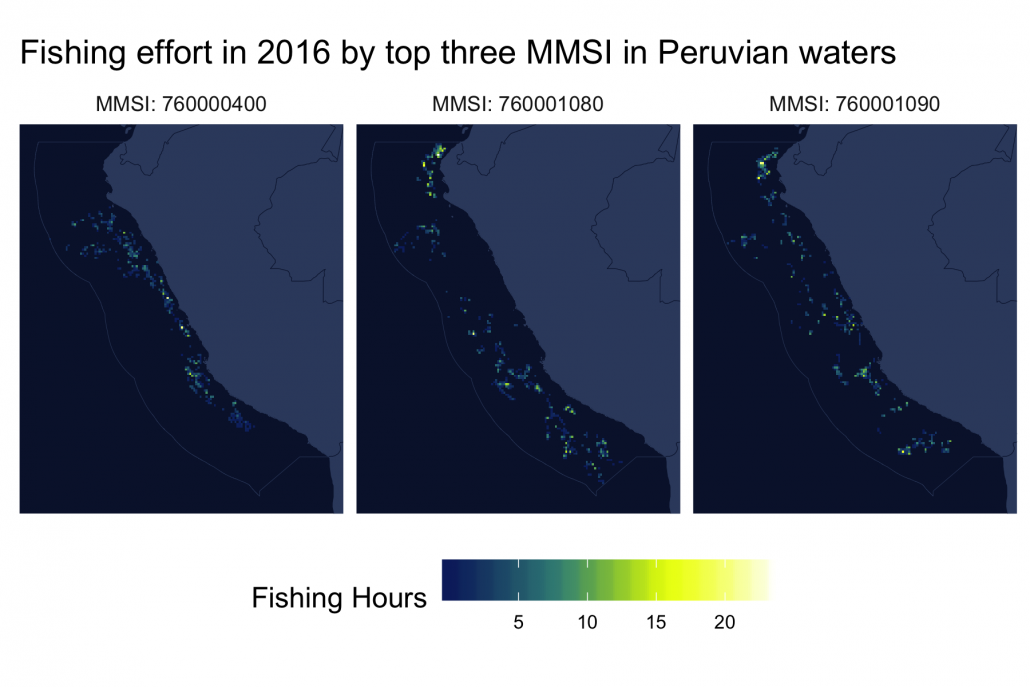
Lastly, by joining this data with the fishing vessel data we are able to pull out the information for each MMSI.
# load fishing vessel effort data
fishing_vessels <- read_csv('~/data/gfw-public-data/fishing_vessels/fishing_vessels.csv')

# Join vessel details to Peruvian mmsi
per_mmsi <- left_join(per_mmsi, fishing_vessels)| Metric | 760000400 | 760001080 | 760001090 |
|---|---|---|---|
| tonnage | 1426.72 | 798.17 | 452 |
| length | 60.5 | 60.71 | 45.22 |
| geartype | purse_seines | purse_seines | purse_seines |
| flag | PER | PER | PER |
| fishing_hours | 984.22 | 1497.21 | 1465.42 |
| engine_power | 3173.8 | 1491.5 | 716.16 |
| active_2016 | TRUE | TRUE | TRUE |
| active_2015 | TRUE | TRUE | TRUE |
| active_2014 | FALSE | FALSE | FALSE |
| active_2013 | TRUE | FALSE | FALSE |
| active_2012 | TRUE | FALSE | FALSE |
The fishing vessel information tells us that all three vessels are Peruvian-flagged purse seiners. We can also see each vessel’s length, tonnage, engine power, and whether or not they were active in each year of the data.
Convert to raster and save as GeoTIFF
In many cases, it is desirable to convert the gridded fishing effort data to a raster. Rasters are a standard way of working with gridded spatial data and consist of a matrix of cells (or pixels) organized into rows and columns (or a grid), where each cell contains a value representing information, such as fishing effort. While our public fishing effort data store information calculated in a gridded fashion (e.g. fishing hours per 100th degree cell), the data are provided in long-format .csv files and a conversion is required if you wish to work with rasters.
We can create a single band raster (one data value per cell) by specifying the coordinate variables in our data frame and passing them to the raster::rasterFromXYZ() function along with the variable (e.g. fishing hours) with the values we want to rasterize.
# Select the coordinates and the variable we want to rasterize
effort_all_raster <- effort_all %>%
  dplyr::select(lon_bin, lat_bin, log_fishing_hours)

effort_all_raster <- rasterFromXYZ(effort_all_raster,
                                   crs = "+proj=longlat +ellps=WGS84 +datum=WGS84 +no_defs")
Finally, we can save the raster as a GeoTIFF file with the writeRaster() function by specifying .tif file extension.
# Save GeoTiff
writeRaster(effort_all_raster, filename = 'global_effort_raster.tif')
Conclusion
R is a powerful and popular tool for analyzing and visualizing our public data. In particular, the tidyverse suite of R packages, together with spatial packages like raster and sf, provide numerous handy functions for working with the tabular format of our public data. While there can be a a fairly steep learning curve for R, we hope that this tutorial will help you get started!