When we look at the Global Fishing Watch map, we often see fishing activity that appears to move together. That is, we see groups of vessels consistently fishing in proximity to each other even as the group as a whole moves about the ocean. In other words, we see fleets. Some members of our team, myself included, wanted to know if we could automatically group fishing vessels into these fleets. By understanding fleets, we think we might be able to reveal more about vessel behavior. Maybe we can tell what types of species a vessel is targeting. Or, if a vessel is in a fleet where other vessels have labor violations or illegal behavior, it might indicate a higher chance that our particular vessel has a higher risk of these infractions.
The overall approach to grouping these vessels into fleets is clear: use one of the many clustering methods to group vessels. However, turning this general approach into an algorithm that creates realistic fleets requires some experimentation. In this blog post, I present an overview and motivation for the approach we used. For the gory details, take a look at one of the notebooks located in https://github.com/GlobalFishingWatch/fleet-clustering/.
Clustering by Day
The first order solution is to start with one point from each vessel per day and create a vessel cluster for each day as shown below. I use HDBSCAN for the clustering because it is one of the few clustering algorithms that doesn’t require the number of clusters to be specified in advance, and because I’ve had good luck with it in the past.
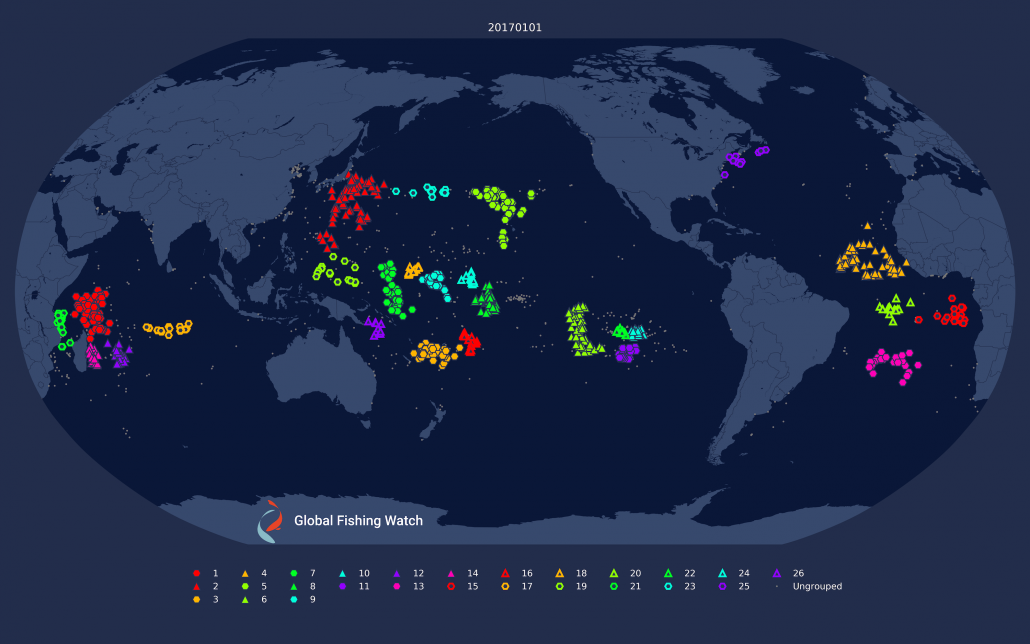
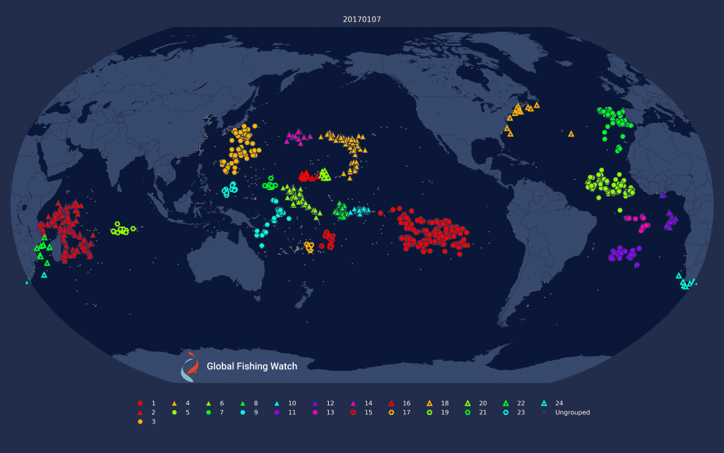
Figure 1: Daily clustering applied to drifting longliners on the 1st and 7th of January, 2017. Note how some of the clustering changes dramatically; notably in the eastern Pacific and around Madagascar.
There are several problems with this approach which Figure 1 helps make clear. First, clusters are not necessarily consistent across days, and each day can have a different set of “fleets.” Second, fleets can break into smaller clusters on different days, making it difficult to clearly define what a fleet is.. Third, not all vessels broadcast every day, which means they won’t be clustered on some days.
It’s possible to link clusters across days by looking at the overlap between fleets, and in fact I reuse this idea later when linking clusterings across years, but this doesn’t help with the second two issues. Fortunately, there’s a better solution: clustering across both space and time.
Clustering Across Space and Time
Clustering over an extended period of time — I used one year — fixes most of the issues with clustering a day at time. HDBSCAN supports passing a matrix of distances between pairs of objects rather than object locations. This allows computing the average distance between vessels over the year and passing that in as the distance matrix. By omitting any days from the average when a vessel in a pair wasn’t broadcasting, issue number three is almost completely avoided. I say almost because there is one remaining corner case: if two boats never broadcast on the same day the average is not defined. Fortunately, HDBSCAN also allows passing in a special missing value for some distances and will still sensibly cluster objects as long as there aren’t too many missing values.
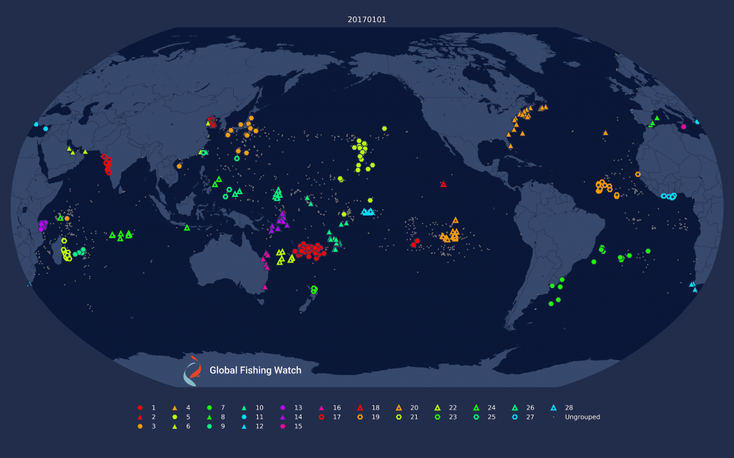
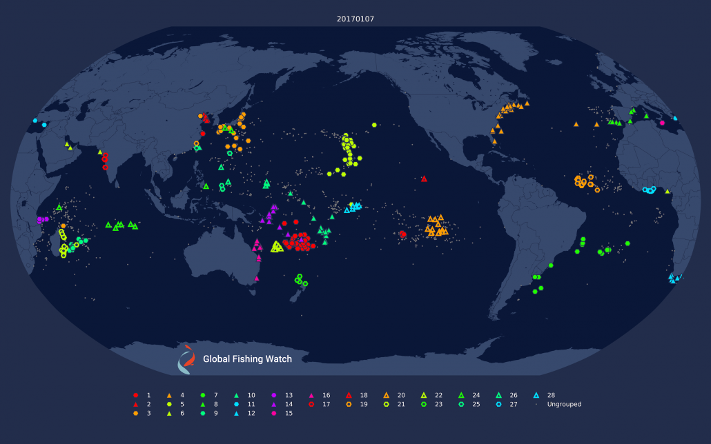
Figure 2: Results of yearly clustering applied to drifting longliners shown on the 1st and 7th of January, 2017. The clustering is now consistent across dates, but many fewer boats are clustered because the clustering is too strict.
Because we are clustering over an entire year, the clusters are consistent across time. A fleet is the same fleet on January 1 as it is on December 31. For clustering over longer intervals, see the section on Stitching Fleets Together Across Time at the bottom of this post.
Clustering across across time like this also results in clusters where vessels are consistently together. In fact, it is rather too good at this, only clustering vessels that spend nearly all of their time together. This ends up missing a lot of vessels, because vessels often leave their fleet for a time to return to port or just for short excursions to other fishing grounds. This is visible in the new clusterings shown in Figure 2 where the number of clustered vessels is far fewer than in the previous daily clusterings. Fortunately, since we are already computing a custom distance matrix by hand, we can do better by redefining what we mean by average distance.
Tweaking the Distance Matrix
The initial distance matrix computed the root-mean-square (RMS) value of the Haversine distance (which is a fancy way of saying “distance between points on a sphere”) between each pair of vessels. By adjusting the way the average distance is computed it is possible to get the clustering to produce much more realistic fleets. We have now reached the point in the narrative, where it is traditional to sweep a great deal of experimentation under the rug. Let me just say that I tried:
- Capping the individual distances before averaging.
- Averaging only the N closest days for each vessel pair.
- Trying different averaging methods, notably the geometric mean.
- Sorting the list of distances for each vessel pair then weighting the average based on position in the list.
These are just the approaches that worked well enough that I recall them, I’m sure there were quite a few more that I’ve forgotten that were complete flops.
In the end I arrived at a combination of (3) and (4) that does a good job of clustering vessels into realistic fleets. For each pair of vessels, the Haversine distances are computed on each day, then the distances di are sorted into increasing order and the overall distance is computed as the weighted geometric mean of the distances, specifically:
[latex]d=exp(\frac{1}{N} \sum_{0}^{N-1})log(d_{i})W_{i}[/latex]
Where N is the number of days with defined distances and Wi is a weight factor defined by:
[latex]W_{i}=(\frac{N_{year-i}}{N_{year}})^{2}[/latex]
Where [latex]N_{year}[/latex] is the number of days in the given year (365 or 366 if it’s a leap year).
This averaging scheme may appear arbitrary, but it follows naturally from the form of the problem. First, note that the geometric mean has an effect similar to capping the distances, in that it weights smaller distances more than larger distances. To appreciate this, consider the geometric, vs arithmetic means of 1 and 10,000: the geometric mean is ~100, while the arithmetic mean is ~5,000. There is a similar connection between (4) and (2). We can can recast (2) as sorting the distances and then computing a weighted average with the first N having a weight of 1 and the rest a weight of 0. The procedure in (4) is very similar except that the weights vary smoothly from 1 to 0. Having established that (3) and (4) are in some sense smooth analogues of (1) and (2), let’s discuss why the later make sense in the context of clustering fleets.
The rationale for (1), and by extension (3), rests the fact that beyond a certain distance a vessel is simply away from the fleet. A vessel that is 2000 km away from the fleet is not significantly less associated with the fleet than one that is 1900 km away. In contrast, the difference between vessels that are 110 km and 10 km away is large in terms of likelihood of fleet membership. Both capping the distances and using the geometric mean are ways to codify this and in practice the latter performed better.
Similarly, the rationale for (2) and (4) rests on the fact that vessels don’t need to be together for the entire year to be considered part of one fleet since vessels leave to visit port or for other short excursions. This can be taken into account by only considering the N closest days as done in (2). However, this requires tuning on N, the best value of which may vary significantly from region to region, and in practice the continuous version of this concept, expressed in (4) seems to perform better. There are an infinite number of weighting functions that can be used here though, so there is still plenty of opportunity for tuning.
Clustering vessels using this approach yields fleets that are consistent across time, at least on a yearly time scale, but has coverage similar to the daily clusters as show below. The clusters tend to correspond to specific flag states, which lends credence to them representing real fleets. More importantly, the resulting fleets appear realistic and offer useful insights into vessel movement.
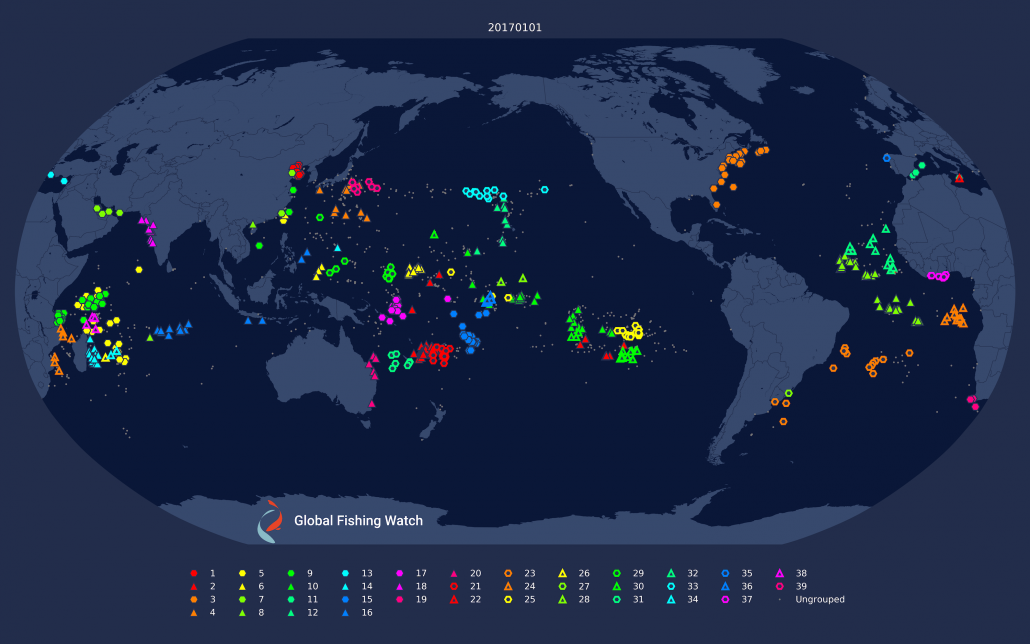
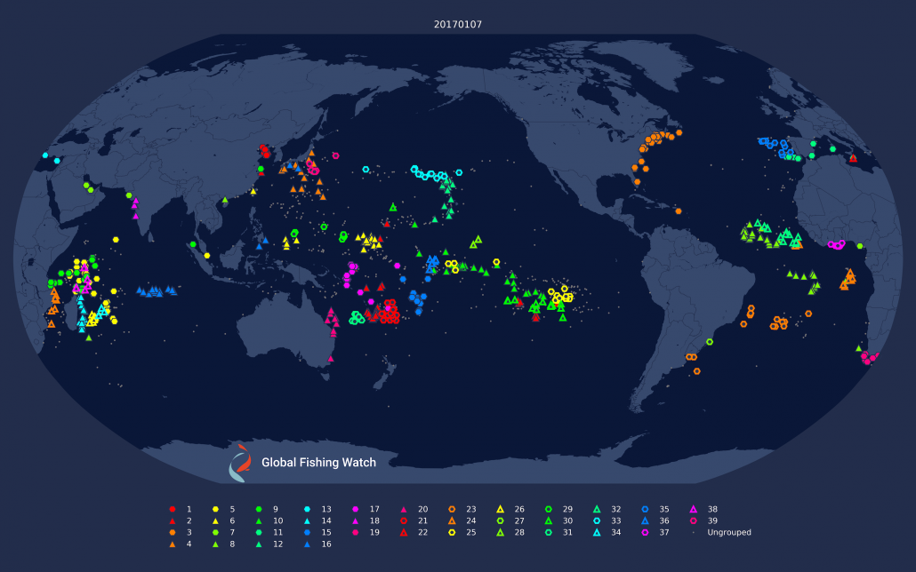
Figure 3: Results of yearly clustering applied to drifting longliners with a custom distance metric shown on the 1st and 7th of January, 2017. The clustering is still consistent across dates, but now clusters a much larger fraction of the boats. The resulting clusters are also more fine grained.
Stitching Fleets Together Across Time
The clustering method described above does a nice job clustering vessels over a one year, but how should we go about clustering vessels across longer time frames? The obvious answer is to just extend the time range used in the clustering technique above. However, this has two issues. The first is just convenience. Using a longer time scale requires a new set of experiments to find the correct clustering parameters, and running the clustering over the longer time range is slower, meaning finding these parameters takes longer than it did the first time around.
The second issue is what I’m calling the fleet coherence time. Vessels don’t remain attached to the same fleet forever. There is some turnover as boats are sold, reflagged, or repurposed, so one would like a solution that allows fleet membership to evolve over time. Our current solution is to cluster years separately, but allow hints about fleets to pass between years, and then stitching the fleets together across years.
Stitching the fleets together is relatively straightforward. I use the fleets from 2017 – the year that I did my parameter tuning on – as the canonical fleets. I then match fleets from subsequent and previous years to these fleets my maximizing the intersection-over-union (IOU). There are two corner cases: first, in some cases, multiple clusters will match a single fleet, in which case they are merged. Second, some clusters may not match an earlier fleet at all, in which case they are dropped.
Just stitching the fleets together in this way, is not quite enough to get well behaved, consistent fleets because some of the clusterings change too much year to year. The most egregious example is the set of fleets around Madagascar. Small differences in the vessel distribution can change the clustering of these fleets from a group of six or so fleets to a single fleet. Which of these representations is preferable depends on ones application, but one would prefer it to stay stable. My current solution is to add a fleet based pseudo distance to the average distance computed above. The pseudo distance is computed based on the fleets found in 2017 and this distance is added to the base distance computed for 2016 and 2018 to stabilize the fleets from those years. This approach is a bit ad hoc, but in practice it seems to work well.
Figure 4: Results of yearly clustering applied drifting longliners with a custom distance metric for 2016 through 2018
To fully appreciate the fleet clustering it helps to see how the vessels behave over an extended period of time as shown in Figure 4. Additionally, there are fleet animations for drifting longliners, trawlers, purse seines and squid jiggers available in the repo for this project https://github.com/GlobalFishingWatch/fleet-clustering/.